
You probably know that person at work who’s a pro at Microsoft Excel. Give them a spreadsheet, and in no time, they’ve delivered a professional report with impressive charts, tables and Sparklines.
Better yet, they know how to use one of the most powerful features in Excel, the PivotTable, to count things, group data in ranges, and drill down to extract the data behind any total.
You wish you had their Excel skills.
Over the years, you’ve struggled to analyze your data in Excel, look for patterns, and share important information in an easy-to-understand report or chart.
So, what can you do to improve your Excel skills and not keep asking your in-house Excel expert for help?
Thanks to a new infographic from Excel Training, you can soon be on your way to becoming an Excel power user at work.
Start by learning charting, move on to conditional formatting for highlighting, discover how the Quick Analysis tools can speed up creating charts, and yes, get tips on using PivotTables to analyze worksheet data.
Take a look at the infographic to learn seven tips for working with Excel. If you prefer to read, check out the text version of the infographic.
Source: 7 essential Excel tricks every office worker needs to know by Excel Training
7 Tips for Sharpening Your Excel Skills
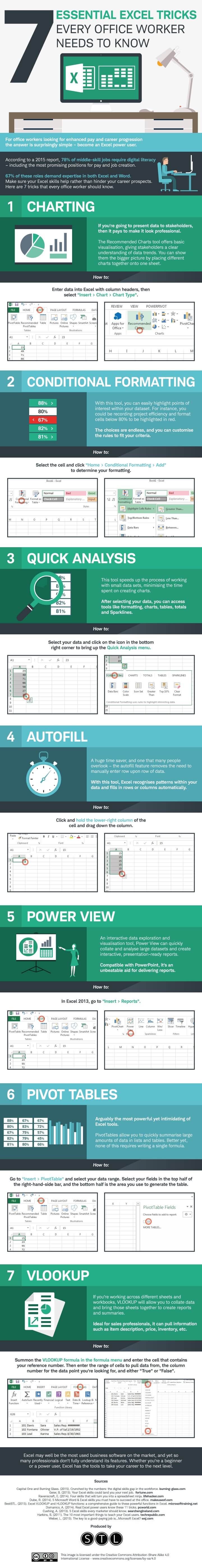
For office workers looking for enhanced pay and career progression, the answer is surprisingly simple—become an Excel power user.
According to a 2015 report, 78 percent of middle-skill jobs require digital literacy—including the most promising positions for pay and job creation.
Sixty-seven percent of these roles demand expertise in both Excel and Word. Make sure your Excel skills help rather than hinder your career prospects. Here are 7 tricks that every office worker should know.
1. Charting
If you’re going to present data to stakeholders, then it pays to make it look professional.
The Recommended Charts tool offers basic visualization, giving stakeholders a clear understanding of data trends. you can show them the bigger picture by placing different charts together onto one sheet.
How to: Enter data into Excel with column header, then select Insert > Chart > Chart Type
2. Conditional Formatting
With this tool, you can easily highlight points of interest within your dataset. For instance, you could be recording project efficiency and format cells below 80 percent to be highlighted in red.
The choices are endless, and you can customize the rules to fit your criteria.
How to: Select the cell and click Home > Conditional Formatting > Add to determine your formatting
3. Quick Analysis
This tool speeds up the process of working with small data sets, minimizing the time spent on creating charts.
After selecting your data, you can access tools like formatting, charts, tables, totals and Sparklines.
How to: Select your data and click on the icon in the bottom right corner to bring up the Quick Analysis menu
4. Autofill
A huge time-saver, and one that many people overlook—the autofill feature removes the need to manually enter row upon row of data.
With this tool, Excel recognizes patterns within your data and fills in rows or columns automatically.
How to: Click and hold the lower-right column of the cell and drag down the column.
5. Power View
An interactive data exploration and visualization tool, Power View can quickly collate and analyse large datasets and create interactive, presentation-ready reports.
Compatible with PowerPoint, it’s an unbeatable aid for delivering reports.
How to: In Excel 2013, go to Insert > Reports
6. PivotTables
Arguably the most powerful, yet intimidating of Excel tools.
PivotTables allow you to quickly summarize large amounts of data in lists and tables, Better yet, none of this requires writing a single formula.
How to: Go to Insert > PivotTable and select your data range. Select your fields in the top half of the right-hand-side bar, and the bottom half is the area you use to generate the table.
7. VLOOKUP
If you’re working across different sheets and workbooks, VLOOKUP will allow you to collate data and bring those sheets together to create reports and summaries.
Ideal for sales professionals, it can pull information such as item description, price, inventory, etc.
How to: Summon the VLOOKUP formula in the Formulas menu and enter the cell that contains your reference number. Then enter the range of cells to pull data from, the column number for the data point you’re looking for, and either “True” or “False.”